A Faster Weighted Random Choice

Performing fast random selection with non-uniform weights is trickier than you might imagine.

Estimated reading time: 9 mins

Consider this problem: You have a list of items and a list of their weights. You want to randomly choose an item, with probability proportional to the item’s weight. For these examples, the algorithms will take a list of weights and return the index of the randomly selected item.

Linear Scan

The simplest algorithm works by generating a random number and walking along the list of weights in a linear fashion. This has the advantage of requiring no additional space, but it runs in $O(N)$ time, where $N$ is the number of weights.

def weighted_random(weights):
    remaining_distance = random() * sum(weights)
    for i, weight in enumerate(weights):
        remaining_distance -= weight
        if remaining_distance < 0:
            return i

Linear Scan Demo

This algorithm can be improved slightly by sorting the weights in descending order so that the bigger weights will be reached more quickly, but this is only a constant speedup factor–the algorithm is still $O(N)$ after the sorting has been done.

Binary Search

With a little bit of preprocessing, it’s possible to speed up the algorithm by storing the running totals of the weights, and using a binary search instead of a linear scan. This adds an additional storage cost of $O(N)$, but it speeds the algorithm up to $O(\log(N))$ for each random selection. Personally, I’m not a big fan of implementing binary search algorithms, because it’s so easy to make off-by-one errors. This is a pretty dang fast algorithm though.

def prepare_binary_search(weights):
    # Computing the running totals takes O(N) time
    running_totals = list(itertools.accumulate(weights))
        
    def weighted_random():
        target_distance = random()*running_totals[-1]
        low, high = 0, len(weights)
        while low < high:
            mid = int((low + high) / 2)
            distance = running_totals[mid]
            if distance < target_distance:
                low = mid + 1
            elif distance > target_distance:
                high = mid
            else:
                return mid
        return low

    return weighted_random

Binary Search Demo

Hopscotch Selection

However, it’s possible to do even better by using the following algorithm that I’ve come up with. The algorithm works by first sorting the weights in descending order, then hopping along the list to find the selected element. The size of hops is calculated based on the invariant that all weights after the current position are not larger than the current weight. The algorithm tends to quickly hop over runs of weights with similar size, but it sometimes makes overly conservative hops when the weight size changes. Fortunately, when the weight size changes, it always gets smaller during the search, which means that there is a corresponding decrease in the probability that the search will need to progress further. This means that although the worst case scenario is a linear traversal of the whole list, the average number of iterations is much smaller than the average number of iterations for the binary search algorithm (for large lists).

def prepare_hopscotch_selection(weights):
    # This preparation will run in O(N*log(N)) time,
    # or however long it takes to sort your weights
    sorted_indices = sorted(range(len(weights)),
                            reverse=True,
                            key=lambda i:weights[i])

    sorted_weights = [weights[s] for s in sorted_indices]
    running_totals = list(itertools.accumulate(sorted_weights))

    def weighted_random():
        target_dist = random()*running_totals[-1]
        guess_index = 0
        while True:
            if running_totals[guess_index] > target_dist:
                return sorted_indices[guess_index]
            weight = sorted_weights[guess_index]
            # All weights after guess_index are <= weight, so
            # we need to hop at least this far to reach target_dist
            hop_distance = target_dist - running_totals[guess_index]
            hop_indices = 1 + int(hop_distance / weight)
            guess_index += hop_indices

    return weighted_random

Hopscotch demo

Amortized Analysis

Performing a good amortized analysis of this algorithm is rather difficult, because its runtime depends on the distribution of the weights. The two most extreme cases I can think of are if the weights are all exactly the same, or if the weights are successive powers of 2.

Uniform Weights

If all weights are equal, then the algorithm always terminates within 2 iterations. If it needs to make a hop, the hop will go to exactly where it needs to. Thus, the runtime is $O(1)$ in all cases.

Power of 2 Weights

If the weights are successive powers of 2 (e.g. [32,16,8,4,2,1]), then if the algorithm generates a very high random number, it might traverse the whole list of weights, one element at a time. This is because every weight is strictly greater than the sum of all smaller weights, so the calculation guesses it will only need to hop one index. However, it’s important to remember that this is not a search algorithm, it’s a weighted random number generator, which means that each successive item is half as likely to be chosen as the previous one, so across k calls, the average number of iterations will be <2k. In other words, as the time to find an element increases linearly, the probability of selecting that element decreases exponentially, so the amortized runtime in this case works out to be $O(1)$. If the weights are powers of some number larger than 2, then the search time is still the same, but it’s even less likely to need to walk to the later elements. If the weights are powers of some number between 1 and 2, then the algorithm will be able to jump ahead multiple elements at a time, since the sum of remaining weights won’t necessarily be smaller than the current weight.

These are the two most extreme cases I could think of to analyze, and the algorithm runs in amortized constant time for both. The algorithm quickly jumps across regions with similar-sized weights, and slowdowns caused by variance in weight sizes are offset by the fact that bigger weights near the front of the list (and hence faster) are more likely to be selected when there’s more variance in the weight sizes. My hunch is that this algorithm runs in amortized constant time for any weight distribution, but I’ve been unable to prove or disprove that hunch.

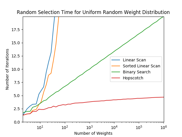
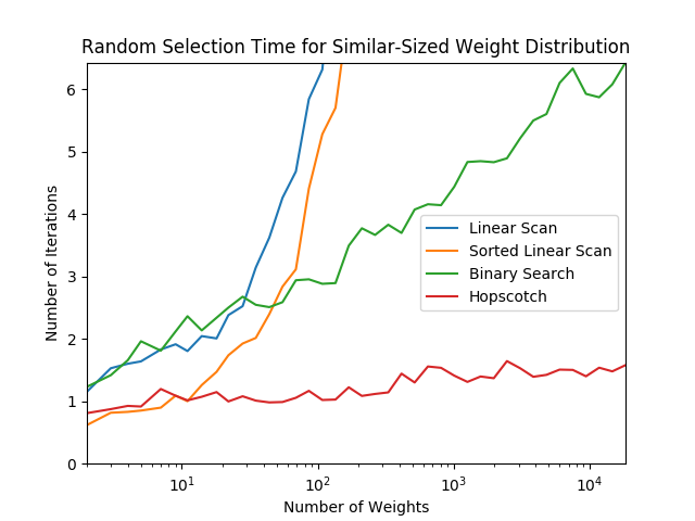
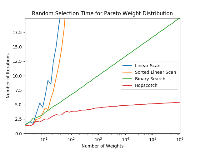
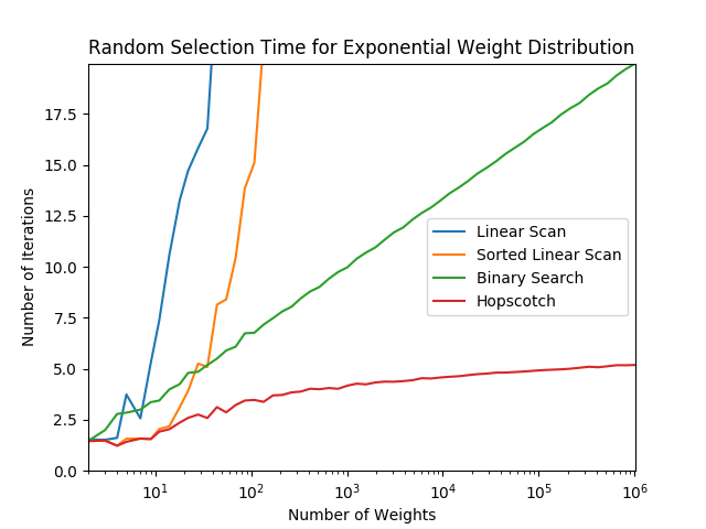
Tests

Here are some tests that show how the different algorithms perform as the number of weights increases, using different weight distributions. The graphs use a logarithmic x-axis, and you can see that the binary search algorithm is roughly a straight line, corresponding to its $O(\log(N))$ runtime, and the linear scan variants have an exponential curve, corresponding to $O(N)$. The hopscotch algorithm looks to me as if it’s asymptotically approaching a constant value, which would correspond to $O(1)$, though it’s hard to say. It certainly does appear to be sublogarithmic though.

Final Words

Python’s random.random() generates numbers in the half-open interval [0,1), and the implementations here all assume that random() will never return 1.0 exactly. It’s important to be wary of things like Python’s random.uniform(a,b), which generates results in the closed interval [a,b], because this can break some of the implementations here.

The implementations here also assume that all weights are strictly greater than zero. If you might have zero-weight items, the algorithm needs to be sure to never return those items, even if random() returns some number that exactly lines up with one of the running totals.

The version of the hopscotch algorithm I present here is the version that I initially conceived, and I think it’s the easiest to grok. However, if your weights do vary by many orders of magnitude, it is probably best to store the running totals from lowest to highest weight, to minimize floating point errors. It’s best to add small numbers together until the running total gets big, and then start adding big numbers to that, rather than adding very small numbers to a big running total. This requires adjusting the algorithm somewhat, but if you’re worried about floating point errors, then you’re probably more than capable of tweaking the code.

If anyone is able to do a good amortized analysis of this algorithm’s runtime for arbitrary weights, I’d love to hear about it. The algorithm is simple to implement and it seems to run much faster than $O(log(N))$. My gut says that it runs in amortized $O(1)$ time, but you can’t always trust your gut.

Addendum: The Fastest Weighted Random Choice Algorithm

There’s one more weighted random algorithm, originally discovered by A.J. Walker in 1974 (described in this excellent page by Keith Schwarz), that I think is the fastest and most efficient algorithm out there. It’s really elegant, and it runs in $O(N)$ setup time, and guaranteed $O(1)$ run time for every random selection. The algorithm is hard to find on Google, despite being relatively simple to implement and clearly better than all other contenders (alas, including my own algorithm), so here is my Python implementation:

You can also see a variant with big and small indices instead of generators. It’s not really faster, but it is easier to port to low-level languages.

def prepare_aliased_randomizer(weights):
    N = len(weights)
    avg = sum(weights)/N
    aliases = [(1, None)]*N
    smalls = ((i, w/avg) for i,w in enumerate(weights) if w < avg)
    bigs = ((i, w/avg) for i,w in enumerate(weights) if w >= avg)
    small, big = next(smalls, None), next(bigs, None)
    while big and small:
        aliases[small[0]] = (small[1], big[0])
        big = (big[0], big[1] - (1-small[1]))
        if big[1] < 1:
            small = big
            big = next(bigs, None)
        else:
            small = next(smalls, None)

    def weighted_random():
        r = random()*N
        i = int(r)
        odds, alias = aliases[i]
        return alias if (r-i) > odds else i

    return weighted_random

Alias Method Demo

For now, I’ll refrain from a full explanation, but essentially, the algorithm works by slicing up the weights and putting them into N buckets. Each bucket gets exactly 1 or 2 of the weight-slices in such a way that the slices in each bucket add up to the same amount, and no slices are left over at the end. The bigger-than-average weights each have small slices get shaved off to fill the gaps in the buckets of the smaller-than-average weights until the big weight is whittled down enough to be smaller-than-average, and the process continues. Why this is guaranteed to works out so perfectly is not immediately obvious, but you can grok it if you spend a while thinking about it and working through some examples.

When you want to do a weighted random selection, you just pick a random bucket (a constant-time operation: buckets[int(rand*N)]) and then choose either the first or second slice in the bucket, with odds proportional to the sizes of the two slices, another constant-time operation: i if (rand*N)%1 <= slice1/(slice1+slice2) else alias (alias is the index of the second slice in the bucket). There’s some really clever optimizations, like always having bucket i’s first slice be from weights[i], and scaling the slice sizes so that the values stored in the bucket always add up to 1. It’s all very clever! Again, please check out and share the more detailed explanation.