Hill Noise

A new approach to random noise generation with novel mathematical properties.

Estimated reading time: 13 mins

Bruce Hill June 1, 2017

Noise functions are a way to produce continuous pseudorandom values across one or more dimensions. The simplest example is a one-dimensional noise function that makes the y-value wobble up and down smoothly, but unpredictably, as you move along the x-axis. It’s also possible to produce 2-dimensional noise, where the amplitude of the noise depends on the x,y coordinates you’re sampling.

This can be used to create hilly terrain in a video game, or more generally, it’s used in computer graphics for procedurally generating textures or making bumpy surfaces. The original version of Minecraft used a 2D noise function to generate heights for terrain as a function of (x,y) coordinates, and later versions used a 3D noise function to generate terrain density as a function of (x,y,z) coordinates to produce overhangs and caves, as Notch describes here.

Existing Noise Functions

There’s many different techniques for making noise. The simplest is called “Value Noise” and it works by generating a set of random points, and then interpolating between them. Most implementations store the random points in a fixed-width array, and points past the end of the array wrap around. Value noise looks like this:

class ValueNoise:
    NUM_VALUES = 256
    SPACING = 10
    def __init__(self, random=random):
        self.values = [random() for _ in range(ValueNoise.NUM_VALUES)]
    def evaluate(self, x):
        # Look up the nearest two values
        x1 = floor(x/ValueNoise.SPACING)
        x2 = ceil(x/ValueNoise.SPACING)
        n1 = self.values[x1 % ValueNoise.NUM_VALUES]
        n2 = self.values[x2 % ValueNoise.NUM_VALUES]
        # Smoothly interpolate between them using cosine interpolation
        k = .5 - .5*cos((x/ValueNoise.SPACING % 1)*pi)
        return ((1-k)*n1 + k*n2)

More commonly, Perlin Noise and Simplex Noise are used. They are slightly more complicated algorithms that rely on similar principles: generate a large amount of random values, then look up and combine those values to get the value at a particular point. However, with Perlin and Simplex noise, the values are used as gradients (partial derivative vectors), rather than heights, which produces slightly better-looking noise.

Fine Details

For many applications, it’s nice to have some extra detail. For example, if you’re using a noise function to make mountains, it’s good to have both “general trend” noise like “go upward for 50 miles, then go downward again”, but it’s also useful to have “local variation” noise like “there’s a bump on the road here”. Commonly, this is achieved by using multiple layers of noise. You start with high-amplitude, slow-changing noise (mountains) and then add smaller, quicker-changing noise (hills), and so on until you get to the smallest level of detail that you care about (bumps in the road). You can use the same noise function for each layer, if you scrunch it up by scaling the input and output of the function. The layers are commonly called “octaves”, and it looks like this:

class OctaveNoise:
    def __init__(self, num_octaves, random=random):
        self.noise = ValueNoise(random=random)
        self.num_octaves = num_octaves
    def evaluate(self, x):
        noise = 0
        for i in range(self.num_octaves):
            size = 0.5**i
            noise += size * self.noise.evaluate(x/size)
        return noise/2

Unfortunately, most of the existing noise functions require pre-generating large amounts of random values that need to be interpolated between (commonly 256). If you keep sampling the noise function far enough in any one direction, the noise function will start repeating itself. Also, most noise functions don’t make any guarantees about the distribution of values. For example, Value Noise picks random points and interpolates between them, but most of the interpolated points are closer to 0.5 than to either 0 or 1, so the distribution of produced values is skewed towards the middle, and it’s quite rare to see the noise function get very high or very low, but quite common to see it pass through 0.5. Perlin Noise and Simplex Noise also suffer from these issues, though they do tend to produce better-looking results than Value Noise. For example, here’s what 1D Simplex Noise looks like:

Notice that the values produced by the Simplex Noise tend to be very heavily biased towards 0.5, and it’s very uncommon to see values close to 0 or 1. (The implementation here is based on the SimplexNoise1234 implementation used in the LÖVE game engine.) For many use cases, it might not matter that the distribution of values is not uniform. In my opinion though, it’s better to have a predictable distribution of values, which can be easily modified to get whatever distribution is desired for your use case.

Hill Noise

As an alternative to address some of these issues, I present a new noise function, which I call “Hill Noise”. It’s inspired by Fourier Decomposition: any periodic function can be broken down into a sum of sine waves of different amplitudes, wavelengths, and offsets. If you generalize the idea, you can create an arbitrarily complex and wobbly function by summing together a bunch of sine waves of different amplitudes, offsets, and wavelengths. If you sum together a bunch of sine waves, then the pattern will only repeat itself after the least common multiple of the periods of the sine waves. For example, the function $f(x) = \sin(2\pi \frac{1}{2} x) + \sin(2\pi \frac{1}{3} x)$ has a period of $6$ . But the function $f(x) = \sin(2\pi \frac{100}{201} x) + \sin(2\pi \frac{100}{301} x)$ has a period of $605.01$ , which is much larger because the two sine waves are slightly misaligned and take a long time to resynchronize. For two sine waves with randomly chosen periods, the resulting function typically has an incredibly large period. Even if the periods aren’t randomly chosen, functions with a very long period can be produced easily. For example: $\sin(2\pi 0.91^0 x) + \sin(2\pi 0.91^1 x) + \sin(2\pi 0.91^2 x)$ has a period of 10,000.

class HillNoise:
    def __init__(self, num_sines, random=random):
        self.wavelengths = [random() for _ in range(num_sines)]
    def evaluate(self, x):
        noise = 0
        for wavelength in self.wavelengths:
            noise += sin(x/wavelength)
        return .5 + .5*noise/len(self.wavelengths)

The result of this is not terribly satisfying, because some of the sine waves are undesirably steep. If we’re trying to mimic the bumpiness of real life things, you typically don’t see bumps in the road that are as tall as a mountain, but as wide as a pebble. Generally, the shorter the length of a bump, the shorter the height of a bump. So, in order to emulate this, instead of $\sin(x/\texttt{wavelength})$ , let’s use $\texttt{wavelength}\sin(x/\texttt{wavelength})$ , which makes the amplitude directly proportional to the wavelength. This concept is similar to the Weierstrass Function, which has the sort of bumpiness we’re looking for.

class HillNoise:
    def __init__(self, num_sines, random=random):
        self.sizes = [random() for _ in range(num_sines)]
    def evaluate(self, x):
        noise = 0
        for size in self.sizes:
            noise += size*sin(x/size)
        return .5 + .5*noise/sum(self.sizes)

It’s a bit unfortunate that this noise function always evaluates to exactly 0.5 at x=0, so let’s introduce some random offsets. (This will be even more useful later.)

class HillNoise:
    def __init__(self, num_sines, random=random):
        self.sizes = [random() for _ in range(num_sines)]
        self.offsets = [random()*2*pi for _ in range(num_sines)]
    def evaluate(self, x):
        noise = 0
        for size,offset in zip(self.sizes, self.offsets):
            noise += size*sin(x/size + offset)
        return .5 + .5*noise/sum(self.sizes)

Now, this function is already pretty useful, and it comes with built-in octaves with different levels of detail. But, ideally it would be nice if you could ask for different distributions of bumpiness. Maybe you don’t care about any noise whose amplitude is less than 0.1, or maybe you want a lot of small noise and a lot of big noise, but not much in between. So, let’s modify the function to take in an arbitrary set of wavelengths:

class HillNoise:
    def __init__(self, sizes, random=random):
        self.sizes = sizes
        self.offsets = [random()*2*pi for _ in range(len(sizes))]
    def evaluate(self, x):
        noise = 0
        for size,offset in zip(self.sizes, self.offsets):
            noise += size*sin(x/size + offset)
        return .5 + .5*noise/sum(self.sizes)

Because we added the random offsets earlier, we can now create two different noise functions with the same wavelengths, but which produce totally different noise! Nice!

So far, this is looking pretty good, but when we throw in a whole lot of sine waves of similar amplitude, they kind of tend to average out and we get a very bland noise function. According to the Central Limit Theorem, randomly sampling points on this noise function will have an approximately normal distribution, and the standard deviation will get smaller and smaller when more sine waves are added. In order to counteract this, we need to use the cumulative distribution function of the normal distribution. Unfortunately, it’s rather tricky to compute the cumulative distribution function, but luckily we don’t need to be very exact, and Wikipedia conveniently has an entire section on numerical approximations of the normal CDF. Using a little bit of math black magic, it’s possible to calculate the standard deviation of the sum of the sine waves, and plug it into the CDF approximation.

class HillNoise:
    def __init__(self, sizes, random=random):
        self.sizes = sizes
        self.offsets = [random()*2*pi for _ in range(len(sizes))]
        self.sigma = sqrt(sum((a/2)**2 for a in self.sizes))
    def evaluate(self, x):
        noise = 0
        for size,offset in zip(self.sizes, self.offsets):
            noise += size*sin(x/size + offset)
        # Approximate normal CDF:
        noise /= sigma
        return (0.5*(-1 if noise < 0 else 1)
                *sqrt(1 - exp(-2/pi * noise*noise)) + 0.5)

The end result of this is noise that is still quite noisy, but now it’s (approximately) evenly distributed between 0 and 1:

With this evenly distributed noise function, it’s fairly easy to create noise with any precise distribution that you want using inverse transform sampling. For example, here’s a Weibull distribution (with adjustable parameters alpha and beta):

class WeibullHillNoise:
    def __init__(self, sizes, alpha, beta, random=random):
        self.hill_noise = HillNoise(sizes, random)
        self.alpha, self.beta = alpha, beta
    def evaluate(self, x):
        u = 1.0 - self.hill_noise.evaluate(x)
        return self.alpha * (-math.log(u)) ** (1.0/self.beta)

That’s quite powerful! And it’s not something that can be easily achieved with just any old noise function.

2D Hill Noise

Now, this is a lovely noise function, but it only works for 1 dimension of input. Let’s expand it to work in 2 dimensions! Instead of summing up sin(x) values, let’s sum up $\frac{\sin(x)+\sin(y)}{2}$ values.

class HillNoise2D:
    def __init__(self, sizes, random=random):
        self.sizes = sizes
        self.offsets = [random()*2*pi for _ in 2*range(len(sizes))]
        self.sigma = sqrt(sum((a/2)**2 for a in self.sizes))
    def evaluate(self, x, y):
        noise = 0
        for i,size in enumerate(self.sizes):
            noise += size/2*(sin(x/size + self.offsets[2*i])
                             + sin(y/size + self.offsets[2*i+1]))
        # Approximate normal CDF:
        noise /= 2*sigma
        return (0.5*(-1 if noise < 0 else 1)
                *sqrt(1 - exp(-2/pi * noise*noise)) + 0.5)

These will be axis-aligned, which is problematic because it will make the noise function much less random-looking, so for each 2D sine wave, let’s rotate its coordinates by a random angle.

class HillNoise2D:
    def __init__(self, sizes, random=random):
        self.sizes = sizes
        self.offsets = [random()*2*pi for _ in range(len(sizes))]
        self.rotations = [random()*2*pi for _ in range(len(sizes))]
        self.sigma = sqrt(sum((a/2)**2 for a in self.sizes))
    def evaluate(self, x, y):
        noise = 0
        for i,size in enumerate(self.sizes):
            # Rotate coordinates
            rotation = self.rotations[i]
            u = x*cos(rotation) - y*sin(rotation)
            v = -x*sin(rotation) - y*cos(rotation)
            noise += size/2*(sin(u/size + self.offsets[2*i])
                             + sin(v/size + self.offsets[2*i+1]))
        # Approximate normal CDF:
        noise /= 2*sigma
        return (0.5*(-1 if noise < 0 else 1)
                *sqrt(1 - exp(-2/pi * noise*noise)) + 0.5)

That looks pretty good, but sometimes the randomly generated rotations are nearly aligned for similar-sized sine waves, and it causes some unfortunate aliasing. Really, we don’t need the rotations to be random, but we want them to be fairly evenly distributed, and similarly sized sine waves should have not-parallel, not-perpendicular rotations. There’s a fairly clever trick for doing almost exactly this task using the Golden Ratio, that I learned about in this blog post about generating random colors programmatically. Let’s use that technique instead of purely random rotations.

GOLDEN_RATIO = (sqrt(5)+1)/2
class HillNoise2D:
    def __init__(self, sizes, random=random):
        self.sizes = sizes
        self.offsets = [random()*2*pi for _ in 2*range(len(sizes))]
        self.sigma = sqrt(sum((a/2)**2 for a in self.sizes))
    def evaluate(self, x, y):
        noise = 0
        for i,size in enumerate(self.sizes):
            # Rotate coordinates
            rotation = (i*GOLDEN_RATIO % 1)*2*pi
            u = x*cos(rotation) - y*sin(rotation)
            v = -x*sin(rotation) - y*cos(rotation)
            noise += size/2*(sin(u/size + self.offsets[2*i])
                             + sin(v/size + self.offsets[2*i+1]))
        # Approximate normal CDF:
        noise /= 2*sigma
        return (0.5*(-1 if noise < 0 else 1)
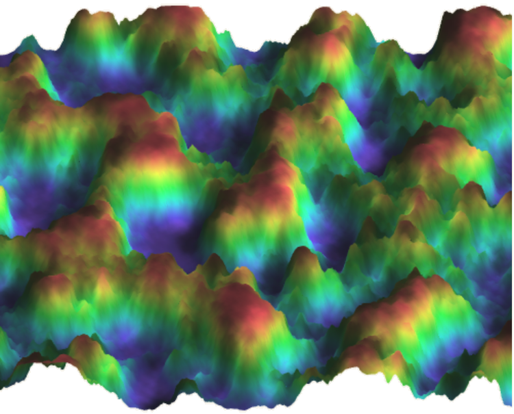
                *sqrt(1 - exp(-2/pi * noise*noise)) + 0.5)

Here’s what the finished product looks like:

3D Hill Noise

Great! Now what about 3D noise? Well… it gets a fair bit more complicated. For one thing, it’s fairly hard to visualize 3D noise, because it has a different value at every point in 3D space. It’s a lot harder to notice if there are any artifacts. So instead, I’m going to visualize it as 2D noise and use time as the 3rd dimension to produce a noise function that wobbles randomly over time. The trick we used for evenly spacing the rotations last time isn’t going to work anymore, because now we need random polar coordinate rotations. With a lot of experimentation, and thanks to the excellent paper Golden Ratio Sequences For Low-Discrepancy Sampling, I managed to come up with a way to generate evenly spaced polar rotations that satisfy the same requirements we had for 2D noise. The end result is starting to get a bit hairy, but it looks like this:

GOLDEN_RATIO = (sqrt(5)+1)/2
class HillNoise3D:
    def __init__(self, sizes, random=random):
        self.sizes = sizes
        self.offsets = [random()*2*pi for _ in range(len(sizes))]
        self.sigma = sqrt(sum((a/2)**2 for a in self.sizes))
    def evaluate(self, x, y):
        fib_num = floor(log((resolution-1)*sqrt(5) + .5)/log(GOLDEN_RATIO))
        dec = floor(.5 + (GOLDEN_RATIO**fib_num)/sqrt(5))
        inc = floor(.5 + dec/GOLDEN_RATIO)
        noise = 0
        j = 0
        for i in range(len(self.sizes)):
            if j >= dec:
                j -= dec
            else:
                j += inc
                if j >= len(self.sizes):
                    j -= dec
            # Convert golden ratio sequence into polar coordinate unit vector
            phi = ((i*GOLDEN_RATIO) % 1) * 2*pi
            theta = acos(-1+2*((j*GOLDEN_RATIO) % 1))
            # Make an orthonormal basis, where n1 is from polar phi/theta,
            # n2 is roated 90 degrees along phi, and n3 is the
            # cross product of the two
            n1x,n1y,n1z = sin(phi)*cos(theta), sin(phi)*sin(theta), cos(phi)
            n2x,n2y,n2z = cos(phi)*cos(theta), cos(phi)*sin(theta), -sin(phi)
            # Cross product
            n3x,n3y,n3z = (n1y*n2z - n1z*n2y,
                           n1z*n2x - n1x*n2z,
                           n1x*n2y - n1y*n2x)
            # Convert pos from x/y/z coordinates to n1/n2/n3 coordinates
            u = n1x*x + n1y*y + n1z*z
            v = n2x*x + n2y*y + n2z*z
            w = n3x*x + n3y*y + n3z*z
            # Pull the amplitude from the shuffled array index ("j"), not "i",
            # otherwise neighboring unit vectors will have similar amplitudes!
            size = self.sizes[j]
            # Noise is the average of cosine of distance along
            # each axis, shifted by offsets and scaled by amplitude.
            noise += size/3*(cos(u/size + self.offsets[3*i])
                             + cos(v/size + self.offsets[3*i+1])
                             + cos(w/size + self.offsets[3*i+2]))

        # Approximate normal CDF:
        noise /= 3*sigma
        return (0.5*(-1 if noise < 0 else 1)
                *sqrt(1 - exp(-2/pi * noise*noise)) + 0.5)

Whew! That’s a heck of a function! But look at the great results!

(The sizes of the sine waves here are generated by $(\frac{i+0.5}{N+1})^{-\log(smoothness)}$ , where $\texttt{smoothness}$ is an adjustable parameter.)

With all of these changes, the resulting Hill Noise algorithm:

Will (practically) never repeat itself.
Has highly configurable characteristics that are easy to understand (sine wave counts and size distributions).
Is memory efficient and easy to implement in a shader, even without access to a pseudorandom number generator.
Produces noise that is (nearly) uniformly distributed across the [0,1] interval.
Can be modified to calculate exact surface normals/gradients.

← Meandering Triangles 6 Useful Snippets →