6 Useful Snippets

A handful of useful programming concepts that can each be implemented in under 20 lines of code.

Estimated reading time: 12 mins

I’d like to present a handful of programming concepts that I find incredibly useful, all of which can be implemented in under 20 lines of code. These techniques can be used in a wide range of contexts, but here, I’ll show how they can all build off of each other to produce a full physics engine in just 75 lines of code.

1. Mixing

The mix() function takes two values and calculates a value some percentage of the way between the two.

Some languages include this as a built-in function (like GLSL), but most don’t, and that’s a shame. Some languages or libraries do include it, but call it “lerp” (short for “linear interpolation”), which I think is a bad name. The core concept of mixing two values is simple, so a simple name is best, and here’s the full implementation:

It’s important to implement mix() the way I’ve presented it, rather than a+amount*(b-a) (the “clever” way with fewer math operations) because the “clever” version is much more susceptible to floating point rounding errors when amount is 1. I’ve encountered this bug before, and it’s a pain in the neck to debug!

def mix(a, b, amount):
    return (1-amount)*a + amount*b

The mix() function is incredibly handy whenever you’re combining two values, but it’s also a great case of self-documenting code. Instead of height = height1 + x*(height2 - height1), you have height = mix(height1, height2, x), which is way more readable! You can also generalize mix() to mix things like vectors or colors, or even mixing between more than 2 things. Applying a function like smoothstep to amount can also give non-linear mixing.

2. Golden Ratio Sampling

Golden ratio sampling is a technique that uses the golden ratio $(\sqrt{5}+1)/2$ (often represented with the Greek phi: φ) to generate values evenly distributed between 0 and 1, where the number of values is not known in advance.

The amount the largest gap is divided by is exactly 1/φ, how cool is that?!

Each new value will be in the largest gap between two previously generated numbers, and each adjacent pair of values will be a fixed distance apart from each other. The trick is to multiply a counter by the golden ratio and take the result modulo one:

GOLDEN_RATIO = (sqrt(5) + 1) / 2
i = 0
def next_sample():
    nonlocal i
    i += 1
    return (i * GOLDEN_RATIO) % 1

Bonus fact: φ-1 = 1/φ. This totally blew my mind when I first learned it!

It’s very broadly applicable, but I often use it for generating colors with different hues, when I don’t know ahead of time how many colors I’ll need. Each new color falls between the two most dissimilar colors yet produced. This blog post goes into more depth. I also used golden ratio sampling when I made Hill Noise because it has a lot of really convenient properties. The paper Golden Ratio Sequences For Low-Discrepancy Sampling goes into more detail and also describes a way to generalize to 2 dimensions and even a handy technique for reverse-engineering an index from a golden ratio sample.

3. Exponential Smoothing

This technique is fantastic for any time you’re trying to get a value to move something towards a target.

If you just want to move at a constant speed, the code is slightly messy (you have to avoid overshooting), but not too complex:

def move_towards(value, target, speed):
    if abs(value - target) < speed:
        return target
    direction = (target - value) / abs(target - value)
    return value + direction * speed

value = move_towards(value, target, 20)

Implemented this way, the movement can have some undesirable properties. First of all, when the value reaches the target, it stops jarringly fast. Secondly, this type of movement has no sense of urgency. It plods along at the same pace, regardless of how far it has to go. This constant pace means that if the target is actively moving away at a speed higher than that constant speed, the target will get further and further away, eventually getting lost. While this might be physically realistic, it’s very undesirable for something like a video game’s camera attempting to follow the character. Exponential smoothing, on the other hand, addresses both of these problems and is even simpler to implement.

If you’re working with a variable-sized timestep and you really care about precision, the general form is mix(value, target, 1-(1-speed)**dt).

speed = 0.1
value = mix(value, target, speed)

Essentially, for every timestep, the value closes a percentage of the distance to the target instead of a fixed amount of distance. Doing it this way is very aesthetically pleasing, and easy to implement, so it’s a great trick to keep up your sleeve.

4. Verlet Integration

Verlet integration is a math technique that can be used for simulating physics and I think it’s severely underrated.

Typically, one of the first things you’ll learn in a game programming tutorial is this technique for simulating motion:

# Euler integration
new_vel = vel + dt*accel
new_pos = pos + dt*new_vel

This is called Euler integration, and it’s only one of many different approximations of how position changes over time. The other approximations have different complexity and accuracy tradeoffs. For example, the Runge-Kutta 4th degree approximation is much more accurate, but is complex to code and slower to compute. However, there’s a third type of integration which is rarely discussed, but which has some amazing properties. It’s called Verlet Integration, and instead of storing position and velocity, you store the current position and the previous position. Assuming you’re using a constant-sized timestep (which you should be doing anyways), the calculation becomes:

# Verlet integration
vel = (pos - prev_pos)/dt
new_vel = vel + dt*accel
new_pos = pos + dt*new_vel

But using substitution, the code above simplifies to:

# Verlet integration (simplified)
new_pos = 2*pos - prev_pos + dt*dt*accel

What’s really useful about this approach is that velocity is implicitly derived from the position and previous position, so if you have to impose constraints on the position, then the correct velocities are automatically calculated! For instance, if you need to keep an object’s position between 0,0 and WIDTH,HEIGHT, the Euler approach would be:

new_pos = pos + dt*vel
if new_pos.x < 0:
    new_pos.x = 0
    if vel.x < 0:
        vel.x = 0
if new_pos.x > WIDTH:
    new_pos.x = WIDTH
    if vel.x > 0:
        vel.x = 0
if new_pos.y < 0:
    new_pos.y = 0
    if vel.y < 0:
        vel.y = 0
if new_pos.y > HEIGHT:
    new_pos.y = HEIGHT
    if vel.y > 0:
        vel.y = 0

With Verlet integration, that whole mess just becomes:

new_pos = 2*pos - prev_pos
new_pos = vec(clamp(new_pos.x, 0, WIDTH),
              clamp(new_pos.y, 0, HEIGHT))

This works for all sorts of constraints, including snapping an object to your mouse, keeping an object on camera, keeping two objects attached to each other, preventing two objects from overlapping each other, and so on. Whatever positional constraints you apply, the velocities will just work themselves out to the correct values.

If you ever need to change an object’s speed, simply modify the previous state value:

prev_pos = pos - desired_vel*dt

A full explanation of Verlet integration is beyond the scope of this post, but Thomas Jakobsen did an excellent writeup for Gamasutra and Florian Boesch also has a great post addressing some issues that can arise.

5. Spatial Hashing

Collision checking is one of the most performance-intensive parts of most games. You need to know when objects collide with each other, but if you have a large number of objects, it takes a lot of time to check for every possible collision. There’s some really efficient techniques for speeding up collision checking, like Quadtrees, Binary Space Partitions, and Sweep-and-Prune. However, many of these are a hassle to implement and are very susceptible to making off-by-one mistakes as you do. Instead, you can get great performance out of a very simple implementation using spatial hashing.

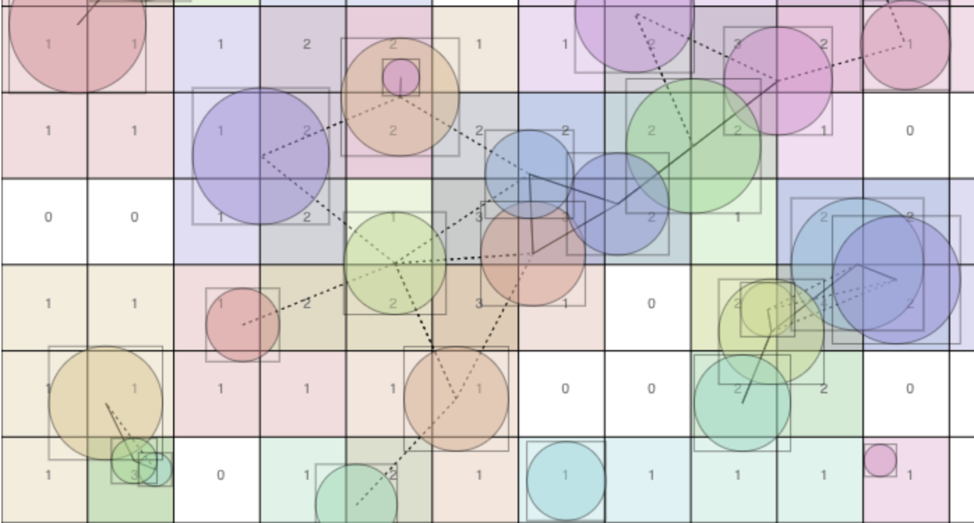
To do collision checking with spatial hashing, you divide the world into large grid cells (buckets). For each object, you find all the buckets that it approximately touches (it’s okay to be overly inclusive, as long as you don’t miss any) and add the object to each bucket’s list of members. As you do, mark the object as potentially colliding with the bucket’s existing members. After processing each object, you’ll have a list of all potential collisions, which you can then process to filter out any false positives (things that fall into the same bucket but don’t actually overlap). For most use cases, this process is very close to linear in speed, because most hash buckets can only fit a couple of objects, and most objects only touch a couple of buckets.

In the demo above, you can see the hash buckets, as well as all the collision checks (lines between circles), most of which are false positives (dashed lines). As the hash buckets get smaller, the number of false positives diminishes, but the number of populated buckets increases. You can drag around the circles to see how they get hashed into different buckets. I chose to use bounding boxes around the circles to find which buckets they might touch because that was easy to implement and fast, but you could be more precise if you wanted to.

Python allows tuples as keys in a dictionary, but in languages that have hash tables but not tuples (e.g. Javascript, Lua), you can use x+","+y (a string key) or x+(GOLDEN_RATIO*y%1) (a floating point key using the golden ratio sampling technique). Or, you could just use a big array and a simple hash function like buckets[(x*K+y)%nbuckets].

def collisions_between(things, bucket_size=100):
    buckets = dict()
    maybe_collisions = set()
    for t in things:
        xmin = int((t.pos.x-t.radius)/bucket_size)
        xmax = int((t.pos.x+t.radius)/bucket_size)
        for x in range(xmin, xmax+1):
            ymin = int((t.pos.y-t.radius)/bucket_size)
            ymax = int((t.pos.y+t.radius)/bucket_size)
            for y in range(ymin, ymax+1):
                if (x,y) not in buckets:
                    buckets[(x,y)] = []
                else:
                    for other in buckets[(x,y)]:
                        maybe_collisions.add((other, t))
                buckets[(x,y)].append(t)

    return [(x,y) for (x,y) in maybe_collisions
            if really_collide(x,y)]

Picking the size of the hash buckets is somewhat arbitrary. The smaller your buckets, the more fine-grained the bucketing is, and the less likely you are to have false positives. However, the smaller the buckets, the more of them there are, so it takes more time to put everything into its buckets and look through the bucket contents. As a rule of thumb, I tend to make my buckets slightly bigger than the size of a median-sized object. That way, most objects will land in between 1 and 4 buckets. However, if precise collision checking is very slow, it might make sense to use smaller buckets to trade off more bucketing time for fewer false positive full collision checks. If it really matters, don’t rely on your intuition, profile the code!

6. Iterative Constraint Solving

Alongside Verlet integration, it’s very useful to be able to solve systems with multiple constraints. A common example would be a constraint that two objects can’t overlap each other, or that all objects must be within the bounds of the screen. In order to solve a constraint, you need to calculate new positions for the objects that satisfy the conditions of the constraint. For a single constraint, this is often very easy (e.g. to solve the “stay on screen” constraint, you simply clamp the position’s values to a specified range).

Things get more complicated when you have to solve multiple constraints. Sometimes solving one constraint causes another constraint to be violated, like if moving an object back on screen causes it to overlap with another object. It may not even be possible to find a solution that satisfies all constraints. So, instead of trying to combine all your constraints together and find a perfect solution, it’s much easier to just try to move incrementally closer to an approximate solution. Here, you can see the “no overlap” and “stay on screen” constraints being solved one at a time:

The stiffness parameter controls how aggressively each iteration attempts to solve each constraint. If the stiffness is at its maximum, each constraint is solved fully on each step, but this can cause a sort of ping-ponging effect when solving one constraint makes another constraint worse, like if one circle is sandwiched between two others. Relaxing the stiffness makes each step move only part of the way towards a solution, which has the effect of making the circles a feel little elastic. With a lower stiffness, the simulation tends to be less erratic, but you might end up with some of the constraints being not fully satisfied (which is bad for rigid objects like rocks, but more realistic for soft objects like people).

This code shows the constraint solving for staying on screen and circular objects not overlapping each other:

def solve_constraints(stiffness=0.5):
    # Solve border constraints
    for thing in things:
        clamped = clamp(thing.pos, vec(0,0), screen_size)
        thing.pos = mix(thing.pos, clamped, stiffness)

    # Solve collision constraints (conserving momentum)
    for a,b in collisions_between(things):
        a2b = (b.pos - a.pos).normalized()
        overlap = (a.radius + b.radius) - a.pos.dist(b.pos)
        a.pos = a.pos - stiffness*a2b*overlap*b.mass/(a.mass+b.mass)
        b.pos = b.pos + stiffness*a2b*overlap*a.mass/(a.mass+b.mass)

The sorts of constraints you can implement are bounded only by your imagination and your ability to write code that takes an incorrect state and outputs a correct state. You can have no-overlap constraints for arbitrary polygons, joint constraints for limbs, hinges, or chains, mouse dragging constraints, path-following constraints, or constraints that make things line up in a tidy grid.

Putting It All Together

Using everything from this tutorial, you can bang together a full physics engine in just 75 lines of code. Here’s my Python implementation (using this simple vector library), and here’s a live Javascript demo that’s basically the same, with a few extra bells and whistles bringing it to ~250 lines:

This is just one way to use these techniques, and I encourage you to look for other creative ways to combine these snippets with other useful ideas. Innovation is almost always the result of combining existing ideas in creative new ways: Hashing + collision detection = spatial hashing, mix() + color = gradients, Verlet integration + iterative constraint solvers = physics engine, golden ratio + color hue = color generator. The snippets presented here are the sort of self-contained ideas that I’ve found to be very good at combining with other ideas.